Spark

This is a hand-in for the Spark assignment of the Big Data course at the Radboud University, Nijmegen.
Back to the blog index.

In this blog post, we look at the internals of the Spark framework.

Docker setup

This blog post uses the docker image andypetrella/spark-notebook with the tag 0.7.0-scala-2.11.8-spark-2.1.0-hadoop-2.7.3-with-hive. The docker image already contains all the necessary programs.

To run the Docker image, simply run:

$ docker run -p 9001:9001 -p 4040-4045:4040-4045 --name sparknb \
	andypetrella/spark-notebook:0.7.0-scala-2.11.8-spark-2.1.0-hadoop-2.7.3-with-hive

Then you can attach a new shell to it using:

$ docker exec -it sparknb /bin/bash

The notebook environment

When the container is up and running, you can navigate to localhost:9001 where you can open a new notebook. You can also check the Spark UI at localhost:4040, where you can find all kinds of system-related information.

Lazy evaluation

As an example, we run the following two lines of code:

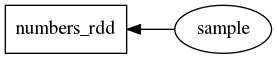
val numbers_rdd = sc.parallelize(0 to 999)
val sample = numbers_rdd.takeSample(false, 4)

In line 1, we create a new RDD with the numbers 0 to 999. In line 2, we request 4 random numbers from that RDD. The sample is shown in the notebook.

The first thing to note is the lazy evaluation that Spark employs. Lazy evaluation is a concept from functional programming languages like Clean which means that data is only computed when it’s needed. This makes it possible to work efficiently with large datasets.

In this case, we can check that Spark used lazy evaluation: if we check the Stages page in the Spark UI after the first line, it is still empty. If we check again after the second line, we see that two jobs have appeared: one for the initialisation step, and one for the sampling step. In other words: had we not requested a random sample, then Spark would not take the time to initialise the data.

Lazy evaluation is not straightforward to implement, especially in impure languages (languages with side effects). In Clean, the expression that is evaluated is stored as a graph on the heap. The run-time system takes care that it is rewritten using the rewrite rules (the functions the programmer writes) until a normal form is reached. This is relatively straightforward, since only one expression needs to be evaluated.

In Spark, it is possible to define variables with dependencies. So, in addition to storing the expression graph of each node, the framework also stores a direct acyclic graph (DAG) with variable dependencies. In the example above, the DAG will look like this:

The DAG of the random sample example

More complex DAGs

The more complex your program, the more complex the DAG that Spark creates for it. Consider the following example (it assumes a text file in /mnt/bigdata/100.txt.utf-8 - you could use something from Project Gutenberg, for example):

val lines = sc.textFile("/mnt/bigdata/100.txt.utf-8")
println("Lines:\t", lines.count)
println("Chars:\t", lines
	.map(s => s.length)
	.reduce((a,b) => a + b))
val wc = lines
	.flatMap(line => line.split(" "))
	.filter(_ != "")
	.map(word => (word, 1))
	.reduceByKey(_ + _)
wc.takeOrdered(10)

Several things are happening here. First, we read a text file. We print the number of lines in it. Using a simple map-reduce, we sum the lengths of all the lines to print the number of characters. Then, we find the 10 most frequently used words with another map-reduce task.

To do wordcount, we first flat-map a split operation on the lines. We use a flatMap instead of a map, because every input element yields a list of output elements. The type of map is (a -> b) [a] -> [b], whereas the type of flatMap is (a -> [b]) [a] -> [b]. That is, flatMap = flatten o map. Since split returns a list, and we don’t need to keep data grouped by lines, we use flatMap.

All the words found are filtered to remove the empty word. We then create tuples from it to include a count (initially 1). We reduce by key using the addition operator to sum all the counts per word. With takeOrdered, we get the ten highest results, ordered by value - i.e., the ten most frequent words and their usage count.

The DAG for this complete example looks like this:

The DAG of the wordcount example

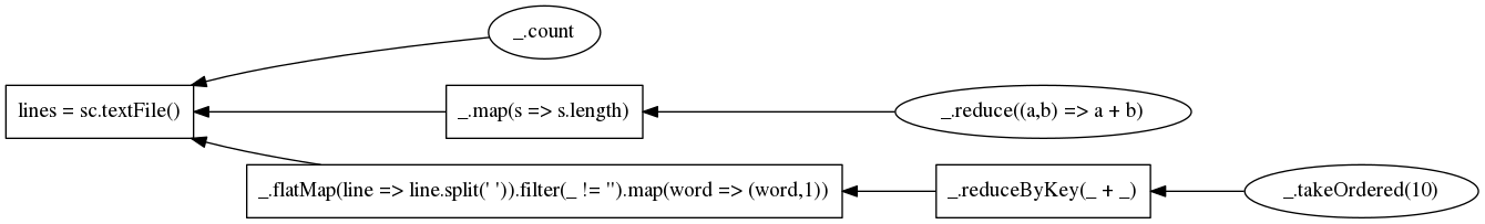
A couple of things should be noted here.

Stage merging

We see that three Scala operations have been merged into one stage in the DAG. This is possible, because the data can be streamed through this operation (no shuffling or sorting is needed). Spark creates one new RDD, to which words are added iff non-empty and with an additional number (initially 1). This instead of creating three RDDs:

One with all words
One with all non-empty words
One with tuples of all non-empty words and the number 1

This saves computation time and memory. It is handled by Spark’s internal DAG optimiser. This is actually a rather fancy tool. It also supports things like predicate pushdown. This means that operations like filter are moved up in the pipeline when possible. So, had we written the following:

val wc = lines
	.flatMap(line => line.split(" "))
	.map(word => (word, 1))            // First map
	.filter(_._1 != "")                // Then filter
	.reduceByKey(_ + _)

Then the Spark DAG optimiser would have recognised that it is more efficient to filter first, and only map those elements that have not been filtered out.

Caching

We also note that we now have a node that is needed by multiple child nodes. Now, suppose that after counting the number of lines, we (or another user on the same cluster) performs some memory-intensive operation. Spark may then decide to remove the lines RDD from memory. This is possible, because it can recreate it by following the DAG. (In this case, we only need to reread the text file, but had the trail for lines contained computations then we would have had to redo those as well.)

In this case, as a programmer, we know that we will reuse lines and that it is therefore a bad idea to remove it from memory. We can hint Spark that it should try to keep it in memory as long as possible, by calling lines.cache(). This by no means is an imperative, it is merely a suggestion to Spark.

Learning from Spark’s recomputations

Certain aspects of Spark’s memory management (in particular, the idea to recompute instead of store) have applications in programming language design.

Let’s take the functional language Clean as an example. At run-time, a graph store is kept in memory that describes all the nodes in the DAG that is your program. A stack of nodes describes which nodes are currently under reduction. We only need to have access to the nodes on the stacks and their children. All the other nodes are considered garbage (they can never be used) and will be removed by the garbage collector when memory is full. This works more or less as follows:

The memory is divided into two semispaces, left and right. When the current, say the left, semispace is full, the garbage collector first copies the top of the stack to the right semispace. It proceeds to copy its children, grandchildren, etc. to the right semispace as well. When this is finished, the garbage collector does the same for the next element on the stack, etc., until all needed nodes have been copied. Then, the garbage collector marks the whole left semispace as unused.

At some point, it may be the case that almost all nodes need to be kept in memory. Then, the copying collector takes a lot of time to copy all nodes to the other semispace, but frees only very little memory, making the program very inefficient. This is currently solved by using other garbage collectors.

Another option would be to intelligently discard part of the memory and instead store a closure describing how to recompute it when needed. As an example, consider these two programs:

Start1 = (hd xs, length xs) where xs = [0..1000000000]
Start2 = (length xs, hd xs) where xs = [0..1000000000]

In Start1, the RTS will first try to reduce hd xs. This is done in O(1). The program then proceeds to compute the length, and the tail-recursive length will do this in linear time and constant space, discarding the part of the list it has seen already.

In Start2 however, the RTS will first compute the length. All this time, the reference to hd, and therefore the whole list, has to be kept in memory until hd xs is reduced. The program will crash, because we cannot keep this list in memory.

In memory, this will look more or less like this after a few iterations of length:

Memory structure of Start2

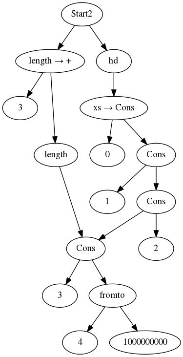
Now, if we rank the nodes in the graph by the length of the path from the root, we will see that the node referenced by the tail-recursive application of length is always on distance 3, and the dot-dot operator (fromto is on distance 4. The nodes that have been seen by length but are still in the graph because of the reference from hd however can potentially have a high distance.

The suggestion here is that we could try, when memory is full, to replace the trail from 0 to the end of the list that has been considered by length with a closure describing that computation. If needed, it can be recomputed (like Spark would do). In this case, it won’t be needed, because hd will discard the tail of its argument. The memory would look like this:

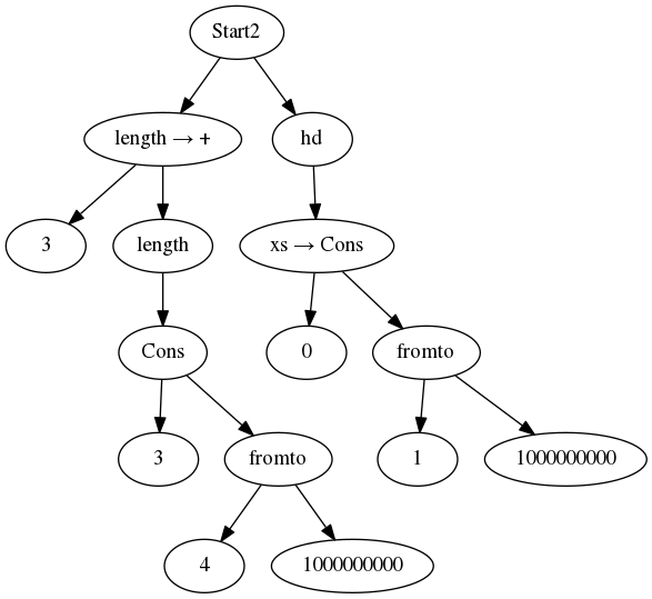
Memory structure of Start2, improved

We see that Start2 can now run in constant space and linear time as well. Yes, discarding data means potentially doing double work (the fromto computation has been doubled). However, everything is better than crashing because the heap is full.

At this point, this remains just a nice idea. More work is needed to invent good heuristics to decide what parts of the graph can be removed with the least risk of doubling work. However, it is clear that ideas from Spark can be applied elsewhere as well.