PART B: Data Mapping

Data reimporting

The data that was saved on disk, must be reimported (and housed in cache) and made into Spark SQL accessible. This was done by:

import org.apache.spark.sql.types._
val addr = spark.read.parquet("file:///opt/hadoop/share/data/addr.parquet").cache()
val kos  = spark.read.parquet("file:///opt/hadoop/share/data/kos.parquet").cache()

addr.createOrReplaceTempView("addr")
kos.createOrReplaceTempView("kos")

spark.sql("SELECT * FROM addr LIMIT 5").show(true)
spark.sql("SELECT * FROM kos LIMIT 5").show(true)

This way we can recheck the composition of data.

Data-table joins

Suppose one wants to know the the kinds of artworks that are located in each of the ‘quarters’ of Nijmegen. For this, the tables (data) from both the datasets needs to be joined logically. For this one could compare (by matching) each of the two coordinate headers that are common to both the tables (('x', 'y') for quarters and ('latitude', 'longitude') for the artworks).

But alas, on a closer inspection of the data, it can be seen that the coordinate systems used in both the tables differ from each other. Hence, an additional mapping step would be needed. The ‘quarters’(BAG) uses the RD system, and the ‘artworks’ uses a more conventional latitude-longitude one. Luckily, there is maven library for this exact kind of conversion. The jar is obtained as follows:

cd /opt/hadoop/share/hadoop/common/lib
echo CTS library...
[ ! -f cts-1.5.2.jar ] \
  && wget --quiet https://rubigdata.github.io/course/data/cts-1.5.2.jar \
  && echo Downloaded CTS library || echo CTS Library already exists

The library was put into a directory on Spark’s CLASSPATH, but the interpreter needs to be restarted for its rediscovery. Addtionally we can make use of it by creating a wrapper class around it called ‘CT’

Serializing code

When non-standard objects within Spark, they have to be ‘serialized’ to be able to send the code to its worker nodes. And the code has been done in CT in such a way that is does exactly that for the easy end-user case.

Coordinate transformation

In order to finally transform from RD to latitude/longitude pairs (WGS:84), a user-defined is made for it using the CT object:

// Register a lambda function that transforms an XY coordinate pair under the name coordMapper
spark.udf.register("coordMapper", (x:Float, y:Float) => CT.transformXY(x,y))

and it can be used with the Zeppelin Notebook’s %spark.sql directive directly as follows, to get all the transformed coords, of the streets in which there are people living:

-- Toernooiveld with its coordinates after transformation from RD New to WGS:84
select street, quarter, coordMapper(x,y) latlon from addr where street == "Toernooiveld"

TSV file

More %spark.sql directive

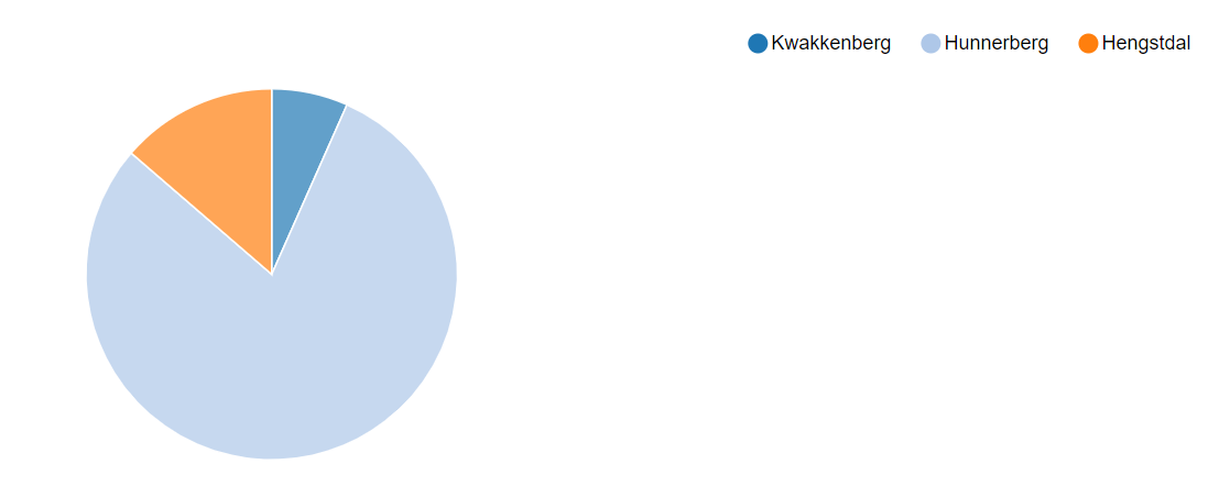
1. Berg en Daak street spans multiple quarters (it is very long). To find the number of people living in the street, but belonging to different quarter, one can use the following and switch to a ‘pie chart’ representation.

   select quarter, count(quarter) from addr where street == "Berg en Dalseweg" group by quarter
   

   giving this figure

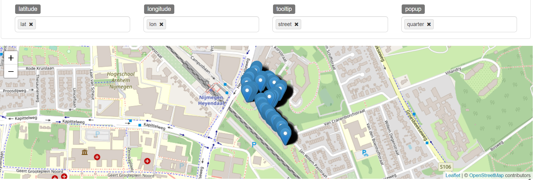
2. To view the addresses of ‘Toernooiveld’ on a map, one can make use of the Map extension of Zeppelin (zeppelin-leaflet), after flatten-out the two columns of the previous latlon column as follows:

   select street, quarter, latlon._1 as lat, latlon._2 as lon
   from ( select street, quarter, coordMapper(x,y) as latlon from addr where street = "Toernooiveld")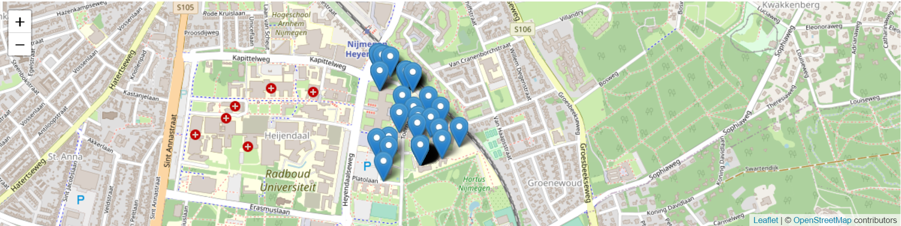
   

   

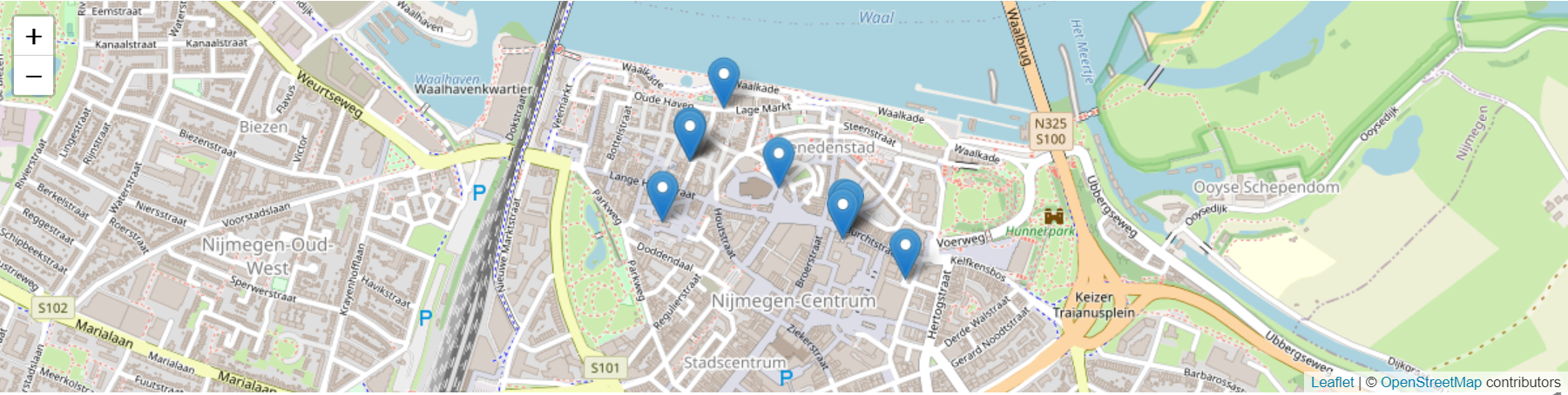
3. To view the adresses of my own street ‘Professor Bromstraat’, “Toernooiveld” in the previous example, was simply replaced by “Professor Bromstraat”.
   

Finally, joining them

A transformation of coordinates is applied onto the artworks dataset as every artwork has an address, which is to be matched to an address in the addresses dataset, and not the other way around. So, the addresses dataset will be joined to (will be the incoming table) the artworks one. So, in order to not perform processing to the incoming data, chosing to instead, do the transformation processing to the in-situ data is a better option.
For this purpose, we introduce (register) a new function (lambda) and use it:

spark.udf.register("transformLatLon", (lat:Float, lon:Float) => CT.transformLatLon(lat,lon))

and use the spark.sql directive for the rest again:

-- Artworks with XY coordinates (transformed using the lambda above)
create temp view kosxy as
select naam, bouwjaar, latitude, longitude, XY._1 as x, XY._2 as y 
from ( select naam, bouwjaar, latitude, longitude, transformLatLon(latitude, longitude) as XY from kos )


-- limiting to 10 results
select * from kosxy limit 10


-- Join addresses and artworks on location
create temp view kosquarter as
select distinct naam, quarter, first(latitude), first(longitude), min(bouwjaar) as jaar from kosxy, addr
where abs(kosxy.x - addr.x) < 10.0 and abs(kosxy.y - addr.y) < 10.0
group by naam, quarter


-- The ten oldest artworks
select * from kosquarter order by jaar asc limit 10

Final result

Growth of Nijmegen

Is it possible to prove that Nijmegen, as a city, grew through the years, in the years that the artworks were created in? The painting that was made the earliest min(bouwjaar) from a list of the paintings belonging to each of the coresponding quarter, can be taken into consideration as:

select distinct quarter, min(jaar) as jaar from kosquarter group by quarter order by jaar

giving this

But some of the quarters seem to be missing from the list. Ofcourse, because not all quarters had a painting made in them! We can easily get a number for the ‘missing artworks’ by:

spark.sql("select count (distinct naam) from kos where naam not in (select naam from kosquarter)").show()

giving a number of ‘138’.

Own analysis

1. To see which all quarters never ‘produced’ an artwork, the following was used:

   select  distinct locatie  from kos   where naam not in (select naam from kosquarter)
   

   giving this list